Recntly I found myself needing to implement more advanced control flow in some models I have been hacking on in my job at Rubyroidlabs – software development company and Railscarma. In past I never really needed any graph conditionals or loops or any combinations thereof, so I had to dive into documentation and read up on them.

This blog post covers tf.cond and tf.while_loop control flow operations and was written to document and share my experience learning about them. Both of the operations seem intuitive on the first look, but I got bitten by them so I wanted to document their usage on practical examples so I have something as a reference I can return to in the future should I need to. It is easy to use this article to eCommerce software development niche.

tf.cond: simple lambdas

This is basically a slightly modified code from the official documentation. Here we have two constant tensors t1 and t2 and we execute either f1() or f2() based on the result of tf.less() operation:

1 2 3 4 5 6 7 8 9 10 t1 = tf.constant(1) t2 = tf.constant(2) def f1(): return t1+t2 def f2(): return t1-t2 res = tf.cond(tf.less(t1, t2), f1, f2) with tf.Session() as sess: print(sess.run(res))

As expected the printed number is 3 since 1<2 and thus the f1() gets executed. It’s worth noting that both lambdas here are single line functions, neither of which accepts any parameters.

tf.cond: parametrised lambdas

Now if you want to pass some values into the f1() and/or f2() lambdas defined earlier, you need to write a simple closure that encloses the passed in parameter i.e. something like this:

1 2 3 4 5 6 7 8 9 10 11 12 13 14 15 16 17 def f1(p): def res(): return t1+t2+p return res def f2(p): def res(): return t1-t2+p return res t1 = tf.constant(1) t2 = tf.constant(2) p1 = tf.constant(3) p2 = tf.constant(4) res = tf.cond(tf.less(t1, t2), f1(p1), f2(p2)) with tf.Session() as sess: print(sess.run(res))

As expected the above code will print 6 since 1<2 and thus the f1(3) gets executed: 1+2+3.

tf.while_loop: basics

Let’s start again with a simple, slightly modified example of tf.while_loop usage borrowed from the official documentation. Once again, we will have two constant tensors t1 and t2 and we will run a loop that will be incrementing t1 while it’s less than t2:

1 2 3 4 5 6 7 8 9 10 11 12 13 def cond(t1, t2): return tf.less(t1, t2) def body(t1, t2): return [tf.add(t1, 1), t2] t1 = tf.constant(1) t2 = tf.constant(5) res = tf.while_loop(cond, body, [t1, t2]) with tf.Session() as sess: print(sess.run(res))

Note that both cond and body function must accept as many arguments as there are loop_vars; in this case our loop_vars are the constant tensors t1 and t2. tf.while_loop then returns the result as a tensor of the same shape os loop_var (let’s forget about shape_invariants for now):

1 [5, 5]

This result makes perfect sense: we keep incrementing the original value (1) until it’s less than 5. Once it reaches 5 the tf.while_loop stops and the last value returned by body is returned as a result.

tf.while_loop: fixed number of iterations

Now if we wanted a fixed number of iterations we would modify the code such as follows:

1 2 3 4 5 6 7 8 9 10 11 12 13 14 def cond(t1, t2, i, iters): return tf.less(i, iters) def body(t1, t2, i, iters): return [tf.add(t1, 1), t2, tf.add(i, 1), iters] t1 = tf.constant(1) t2 = tf.constant(5) iters = tf.constant(3) res = tf.while_loop(cond, body, [t1, t2, 0, iters]) with tf.Session() as sess: print(sess.run(res))

There is a couple of things to notice in this code: * third item in loop_vars is 0; this is the value we will be incrementing * loop incrementation happens in body function: tf.add(i, 1) * once again the returned value (in this particular example) has as many elements as there are in loop_vars

This code prints the following result:

1	`[4, 5, 3, 3]`

First we have the t1 value incremented iters times (3); we don’t modify t2 in this code; the third parameter is the final increment increment value we started with 0 and finished once iters (3) of iterations was reached (this is controlled by cond function).

tf.while_loop: conditional break

With all the knowledge of tf.cond and tf.while_loop we are now well equipped to do conditional loops i.e. writing loops whose behaviour changes based on some condition, sort of like break clauses in imperative programming. For brevity we will stick the code into a dedicated function called cond_loop which will return a tensor operation we will run in the session.

This is what our code is going to do: * we will be looping fixed number of loops set by iters * in each loop we will increment our familiar constant tensors t1 and t2 * in the final loop, we will swap the tensors instead of incrementing them

You can see this in the code below:

1 2 3 4 5 6 7 8 9 10 11 12 13 14 15 16 17 18 19 20 21 22 23 24 25 26 27 28 def cond_loop(t1, t2, iters): def cond(t1, t2, i): return tf.less(i, iters) def body(t1, t2, i): def increment(t1, t2): def f1(): return tf.add(t1, 1), tf.add(t2, 1) return f1 def swap(t1, t2): def f2(): return t2, t1 return f2 t1, t2 = tf.cond(tf.less(i+1, iters), increment(t1, t2), swap(t1, t2)) return [t1, t2, tf.add(i, 1)] return tf.while_loop(cond, body, [t1, t2, 0]) t1 = tf.constant(1) t2 = tf.constant(5) iters = tf.constant(3) with tf.Session() as sess: loop = cond_loop(t1, t2, iters) print(sess.run(loop))

The main difference between this code and the code we discussed previously is the presence of tf.cond in the body function that gets executed in each tf.while_loop “iteration” (the double quotes here are deliberate: while_loop calls cond and body exactly once). This tf.cond causes body to execute swap lambda instead of increment at the end of the loop. The return result confirms this:

1	`[7, 3, 3]`

We set out to run 3 iterations which will increment the constants 1 and 5 in each iteration except for the last one when we swap both values and return them along with the iteration counter. (1+1+1, 5+1+1 <-> 7, 3).

Summary

TensorFlow provides powerful data flow control structures. We have hardly scratched on the surface here. You should definitely check out the official documentation and read about things like shape_invariants, parallel_iterations or swap_memory memory parameters that can speed up your code and save you some headaches. Happy hacking!

TensorFlow Dataset API Exploration Part 1

I’ve been working on a small project of mine in TensorFlow (TF) recently when I noticed how increasingly annoyed I get every time I need to write some data pipeline code. Dealing with TF queues, external transofmration libraries or whatnot felt a bit clunky and a bit too low level to my liking, at least as far as the API abstractions are concerned, anyways.

Keeping en eye on TF development, I’ve been aware of the tf.contrib.data.Dataset API which has seen a steady stream of improvements over the past year. I played around with it on and off, but never really got any of my code ported to it. I finally decided to take that step, now that the Dataset API was promoted to stable TF APIs. This post is Part 1 of 2 parts series which explore the Dataset API and highlight some things that either grasped my curiosity or caught me by surprise when I experimented with it.

This post is by no means a comprehensive tutorial. I decided to write it for my own reference so I have it documented all in one place in case I need it. If you find this post useful or notice anything which is not correct, please don’t hesitate to leave a comment below.

Dataset API quick rundown

Based on the official TF programmer’s guide, Dataset API introduces two abstractions: tf.data.Dataset and tf.data.Iterator. The former represents a sequences of raw data elements (such as images etc.) [and/or] their transformations, the latter provides a way how to extract them in various ways depending on your needs. In laymen terms: Dataset provides data source, Iterator provides a way to access it.

Creating Datasets

You can create a new Dataset either from data stored in memory, using tf.data.Dataset.from_tensor_slices() or tf.data.Dataset.from_tensors(), or you can create it from files stored no your disk as long as the files are encoded in TFRecord format. Let’s ignore the on-disk option and have a look at from_tensors() and from_tensor_slices() methods. These are the methods I have found myself using the most frequently.

from_tensor_slices()

According to documentation from_tensor_slices() expects “a nested structure of tensors, each having the same size in the 0th dimension” and returns “a Dataset whose elements are slices of the given tensors”. If you are as dumb as me, you’re probably a bit puzzled as how to use this method.

The programmer’s guide shows a couple of simple examples to get you started. The function argument in these examples is either a single tensor or a tuple of tensors. Let’s ignore the single tensor case and let’s have a look at the tuple one:

1 2 3 dataset = tf.data.Dataset.from_tensor_slices( (tf.random_uniform([4]), tf.random_uniform([4, 10], maxval=10, dtype=tf.int32)))

This code will create a dataset that allows to read the data as a tuple of tensors with the following shapes:

1	`<TensorSliceDataset shapes: ((), (10,)), types: (tf.float32, tf.float32)>`

This can be useful for “sourcing” data with labels (1st element of the returned tuple) and its raw data (2nd element). Note how the 0-th dimension becomes irrelevant here: 0-th dimension will be specified by Iterator as we will see in the Part 2 post whcih will deal with it. For now, remember when using from_tensor_slices() what matters is the data dimension and not a number of samples in the sourced data. Like I said, this should become more obvious once demonstrated with Iterator.

If you are like me, you might wonder what happens if you passed in the same tensors as a list as opposed to a tuple i.e. what Dataset gets created using the following code:

1 2 3 dataset = tf.data.Dataset.from_tensor_slices( [tf.random_uniform([4]), tf.random_uniform([4, 10], maxval=10, dtype=tf.int32)])

If you run the above code you will get an exception saying:

1	`TypeError: Cannot convert a list containing a tensor of dtype <dtype: 'int32'> to <dtype: 'float32'> (Tensor is: <tf.Tensor 'random_uniform_83:0' shape=(4, 10) dtype=int32>)`

This suggests that TF does some kind of type safe tensor list “merge”. If you change the second tensor dtype to tf.float32 and try to create the Dataset again, you get a different exception:

1	`ValueError: Shapes must be equal rank, but are 1 and 2`

I had a quick look at TF code and noticed that TF does some kind of tensor flattening and “merging” and since the tensors in the function argument list have different ranks it can’t proceed so it spews the exception. This does not happen if you pass the tensors in as a tuple likr we demonstrated in the first example. This also sort of confirms my initial theory of the type safe “merge”.

Let’s move on and have a look at what happens when we pass in a tuple of tensors of the same shape:

1	`tf.data.Dataset.from_tensor_slices((tf.random_uniform([4,10]), tf.random_uniform([4,10])))`

Now that the passed in tensors have the same shape, TF doesn’t throw any exceptions and creates a Dataset which allows to read the data as a tuple of tensors of the same shape as the ones supplied as a funcion argument:

1	`<TensorSliceDataset shapes: ((10,), (10,)), types: (tf.float32, tf.float32)>`

We can read the data a tuple of tensors with the same dimensions. This can be handy if you source data and its transformation (eg. some kind of variational translation) in the same input stream.

Now, let’s have a look at what happens when we pass in a list of tensors of the same shape:

1	`tf.data.Dataset.from_tensor_slices([tf.random_uniform([4,10]), tf.random_uniform([4,10])])`

What I expected was something similar to the tuple case i.e. I expected a Dataset which would allow to read data in a tuple of tensors, however what TF does in this case is, it creates a Dataset which allows to read a data as a single tensor of the exact same shape as both passed in tensors:

1	`<TensorSliceDataset shapes: (4, 10), types: tf.float32>`

This is different from the tuple case: notice how in this case you read data tensors with predefined shape in both dimensions, whilst in the tuple case the number of read tensors is driven by the Iterator. For now, just take a leap of trust with me and don’t think about it too hard. It will be demonstrated on practical examples in the second part of this series.

The best thing at the end: you can actually name your datasets. The below code is from the official programmers guide, but I’m adding it here for reference:

1 2 3 dataset = tf.data.Dataset.from_tensor_slices( {"label": tf.random_uniform([4]), "images": tf.random_uniform([4, 100], maxval=100, dtype=tf.int32)})

You will get the following Dataset as a result:

1	`<TensorSliceDataset shapes: {label: (), images: (100,)}, types: {labels: tf.float32, images: tf.int32}>`

You can now read your data as dictionaries – super handy for code readability!

from_tensors()

In comparison to from_tensor_slices(), from_tensors() method does not expect its arguments to have the same 0-th dimension. Let’s walk through the same set of examples as earlier.

We’ll start with creating Dataset from a tuple of tensors of different dimensions:

1 2 3 dataset = tf.data.Dataset.from_tensors( (tf.random_uniform([4]), tf.random_uniform([4, 10], maxval=10, dtype=tf.int32)))

We get a dataset which lets us read the data as a tuple, however, the tensors in the returned tuple are different from the from_tensor_slices() case:

1	`<TensorDataset shapes: ((4,), (4, 10)), types: (tf.float32, tf.int32)>`

Notice how the dimensions differ from the the dataset returned by from_tensor_slices():

from_tensors(): (4,), (4, 10)
from_tensor_slices(): (), (10,)

I haven’t really found a use case for this case, but maybe there is one.

Just like in the from_tensor_slices() if we try to create Dataset using from_tensors() by passing in the tensors of different shapes in a list we will get the same error:

1	`ValueError: Shapes must be equal rank, but are 1 and 2`

Now, let’s pass in a tuple of tensors of the same shape. What we get back is the following Dataset:

1	`tf.data.Dataset.from_tensors((tf.random_uniform([4,10]), tf.random_uniform([4,10])))`

TF returns a Dataset which allows to read data as tuples of 2D tensors of the exact same shape (in both dimensions) as the tensors passed in the function argument:

1	`<TensorDataset shapes: ((4, 10), (4, 10)), types: (tf.float32, tf.float32)>`

Once again, notice how this differs from the from_tensor_slices() case:

from_tensors(): (4, 10), (4, 10)
from_tensor_slices(): (10,), (10,)

What’s really interesting, though, is how from_tensors() handles the case when you pass in a list of tensors of the same shape :

1	`dataset = tf.data.Dataset.from_tensors([tf.random_uniform([4,10]), tf.random_uniform([4,10])])`

In this case TF will create a Dataset of 3D tensors. It seems that TF “concatenates” the passed in tensors into one large 3D tensor:

1	`<TensorDataset shapes: (2, 4, 10), types: tf.float32>`

This can be handy if you have different sources of different image channels and want to concatenate them into a one RGB image tensor.

This sums up the Part 1 of the Dataset API explration in the next part we will look at some of the functionality of Iterators.

Summary

tf.data.Dataset provides a nice and concise way of creating data pipelines that can be consumed through tf.data.Iterator . We have discussed different methods of reading data from tensors stored memory. This blog post demonstrated some, to me, unknown or surprising behavior of the Dataset API. In the next part we will look at Iterator API, which should make Part 1 more obvious and understandable. Stay tuned!

Hopfield Networks in Go

As I continue to explore the realm of Artificial Neural Networks (ANN) I keep learning about some really cool types of neural networks which don’t get much attention these days. Many of these networks have not found much practical use in the “real world” for various reasons. Nevertheless, I find learning about them in my free time somewhat stimulating as they often make me think of some problems from a different perspective. One such ANN is called Hopfield Network (a.k.a. Hopfield net), named after its inventor John Hopfield.

In this post I will provide a summary of Hopfield network features which I find the most interesting. I tend to hack on the stuff I learn about, so this post will also introduce my implementation of Hopfield networks in Go which I’ve called gopfield. I used Go again, as I feel comfortable coding in it at the moment, at least until I get a better grasp of TensorFlow. If you find any mistakes in the post or if you find the post interesting don’t hesitate to leave a comment at the end! Let’s get started!

Human memory

Let’s talk about human memory first since Hopfield network models some of its functions. Human memory is an incredibly fascinating and complex thing. When I think about it I often think of the story by Borges called Funes the Memorious. It is a story of man who remembers everything in a crazy amount of detail, a condition also known as Hyperthymesia. Remembering everything we have lived through in so much detail must be ridiculously energy expensive – at least when it comes to recalling stuff from memory. Querying the memory would require some serious “mining” through a tremendous amount of data stored in it.

Most of the people seem to remember mostly the “core features” of the things they experience. We often forget and/or remember things differently compared to how they actually looked or happened. With the help of the brain [neurons], we can assemble experiences from the core features stored in our memory and get a reasonably coherent picture in our minds. This assembly from individual pieces is at the core of the Hopfield network memory model. Let’s explore it a bit more now.

Hopfield network can also be used to solve some optimization problems like travelling salesman problem, but in this post I will only focus on the memory aspect of it as I find it more interesting. Plus, getting the Hopfield network to solve the optimization problems often requires crafting the weights matrix of the Hopfield network manually, which is often quite laborious and generally not easy.

Hopfield network

Hopfield network is a recurrent neural network which can be used as a content addressable memory (CAM). Recurrent neural networks have the ability to maintain an internal state, which makes them a great choice to model various memory functions. This is not to say that Recurrent ANNs are only useful to model memory! Their ability to keep an internal state (i.e. memorize patterns) makes them useful in a wide range of applications, albeit these are often way more complex than Hopfield networks.

Hopfield network consists of binary neurons: they can only be either on or off (0/1 or +1/-1). The neurons are fully connected to each other in both directions i.e. neuron is connected to neuron and vice versa. Each connection has a weight assigned to it. The value of the connection weight is the same in both directions between each two neurons e.g. the weight wij is the same as wji. Network weights can be represented by a weights matrix. Each element in particular row and column of the weights matrix represents the connection weight between those particular neurons. Because of the connection symmetry, the weights matrix is symmetric with diagonal elements equal to 00, since no neuron is connected to itself.

Just like any other ANN, Hopfield network needs to be trained first before it can be used. Unlike some other neural networks, Hopfield network is trained to store data (patterns). Since the Hopfield network neurons are binary, the network only allows to store binary data. There are several ways to train Hopfield networks, but I only focussed on understanding the two most well known training algorithms: Hebbian and Storkey learning.

Hopfield network training stores the binary data [patterns] by modifying the network weights based on particular learning algorithm. Once the network is trained, i.e. it has stored all the data we have supplied to it during training, we can try to recall any of the stored patterns. Before I shed a bit more light on how this process works let’s talk a bit about network energy which can help us understand how Hopfield networks work.

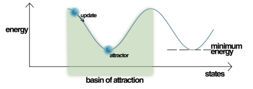
Energy and pattern basins

Energy is a scalar number (measure) which helps to explain and quantify the network behavior mathematically at any point of time. When we store a pattern in Hopfield network during training, it becomes an energy attractor. When we try to recall a pattern from the network by presenting it some data pattern, the stored patterns “attract” the presented data towards them. I will talk about the recollection phase later on, for now just remember that during the pattern recollection the energy of the network changes. If you were to plot the network energy landscape, you would notice that the stored patterns create so called basins of attractions to which the newly presented pattern fall in as you try to recall some pattern

What’s really interesting about the energy function is that it is a Lyapunov function. This is a special kind of function which can be used to analyse the stability of non-linear dynamic systems: something I still remember from the control engineering theory I studied at university. For some dynamic systems Lyapunov function provides a sufficient condition of stability. In the context of a Hopfield net, this means that during the pattern recollection the energy of the network is guarnateed to be lowering in value and eventually ends up in one of the stable states represented by the attractor basins. This means that Hopfield network will always recall some pattern stored in it. Unfortunately the attractors represent only local minima so the recalled pattern might not be the correct one. The incorrect patterns are referred to as spurious patterns (spurious minima).

Open questions

One of the questions which popped up in my head when learning about Hopfield networks was whether there is some way how to actually make the attractor basin deeper. Intuitively, the deeper the attractor basin, the higher the attraction is. One of the options could be doing something like presenting the same pattern to the network during the training multiple times. This way you could “manipulate” the memory by attracting more patterns to this particular “memory”. Equally, if my theory does work, there should also be a way how to do the opposite i.e. “confuse” the memory by making the deep basins more shallow by training the network with some highly correlated but different data patterns: apparently Hopfield network don’t like when the patterns you’re trying to store in it are linearly dependent. I’m not sure any of these theories work. I need to do some research and perform some tests on this. I will report back with the results!

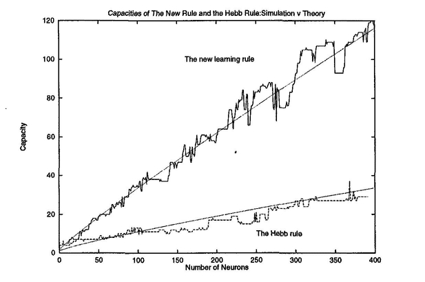
Capacity and spurious patterns

Everything in the nature has its limits and so does the storage of the Hopfield networks. The number of patterns a Hopfield networkcan store is limited by the size of the network and chosen learning algorithm. You can get a rough idea from the graph below

Storkey learning allows to store more patterns than Hebbian learning, however it takes longer to train the network. Hebbian learning on the other hand is simpler and to me personally easier to understand. Either way, if you exceed the network capacity and try to recall a pattern from it, you might experience the spurious patterns I mentioned earlier.

Memory recall

Before we dive into my Go implementation I will shortly describe how the pattern recollection works, because I find it super interesting! During the recall phase the network runs continuously until the states of the neurons in the network settle on some values. Once the energy settles, we are in one of the energy basins. Let’s say we have trained our network using one of the learning algorithms. Now, if we want to recall some pattern we present it to the network. Each neuron si in the network starts switching its state following the formula below:

We know that the network weights are fixed since they are only modified during training, not during the recall phase. This means that the result of the formula above is driven by the states of the neurons in the network. Notice that a neuron switches its state “on” if majority of the neurons the neuron is connected to are also on. The more neurons are in on state, the higher the chance the state of the neurons will switch on, too and vice versa. This seems sort of like a peer pressure. The more of your peers are off, the likelihood you’ll switch off, too is very high. How cool is that? 🙂

So how can this be useful? Imagine you are a police department and you have a database of criminals. When a new crime happens you interrogate a witness and put together a rough image of the offender. This is not an exact image as its based on the witness description. Now you digitize it and run it against the Hopfield network trained with the images of suspects in that area at the given time. The result can give you an indication of who could be the offender. The idea can be expanded to other use cases, like remembering the passwords from a database of known passwords, an idea I have played around in my head for some time.

Go implementation

Thanks for making it all the way to the Go implementation! Let’s dive into some code now! Full source code is available on GitHub. The project codebase is pretty simple. It contains a single Go package called hopfield. You cab create a new Hopfield network like this:Create Hopfield Network

1 2 3 4 5 n, err := hopfield.NewNetwork(pattern.Len(), "hebbian") if err != nil { fmt.Fprintf(os.Stderr, "\nERROR: %s\n", err) os.Exit(1) }

NewNetwork function accepts two parameters: the size of the network and type of the training algorithm. The project currently support only the earlier mentioned Hebbian and Storkey algorithms. Now that you have created new network you can start storing some data in it. The data must be encoded as binary vectors since the Hopfield networks can only work with binary data. The Store method accepts a slice of Patterns. Pattern represents the data as binary vectors. You don’t have to craft the Patterns manually: hopfield package provides a simple helper function called Encode which can be used to encode the data into accepted format. The dimension of the data must be the same as the size of the network:Encode data

1 2 3 4 5 pattern := hopfield.Encode([]float64{0.2, -12.4, 0.0, 3.4}) if err := n.Store([]*hopfield.Pattern{pattern}); err != nil { fmt.Fprintf(os.Stderr, "\nERROR: %s\n", err) os.Exit(1) }

You can store as many patterns in the network as the network capacity allows. Network capacity is defined by both the size of the network and chosen training algorithm. You can query the network capacity or the number of already memorised patterns using the methods shown below:Capacity

1 2	`cap := n.Capacity() mem := n.Memorised()`

Now that you have stored some patterns in the network you can try to recall some patterns from the network using the Restore function. You can specify a mode of the restore (async or sync – Note: restore mode has nothing to do with programming execution) and the number of iterations you want the network to run for:Restore pattern

1 2 3 4 5 res, err := n.Restore(pattern, "async", 10) if err != nil { fmt.Fprintf(os.Stderr, "\nERROR: %s\n", err) os.Exit(1) }

That’s all there is to basics. Feel free to explore the full API on godoc and don’t forget to open a PR or submit an issue on GitHub. Let’s have a look at some practical example.

Recovering MNIST images

Apart from the Hopfield network API implementation, the gopfield project also provides a simple example which demonstrates how the Hopfield networks can be used in practice. Let’s have a quick look at it now! The example stores a couple of MNIST images in the Hopfield network and then tries to restore one of them from a “corrupted” image. Let’s say we will try to “recover” an image of number 4 which has been corrupted with some noise:

The program first reads couple of MNIST images into memory one by one. It then converts them into binary data patterns using a helper function Image2Pattern provided by the project’s API. The images are then stored in the network as vectors which have the same dimension as the number of the image pixels: all the MNIST images from particular set have the same dimension which defines the size of the Hopfield network. Go standard library provides a package that allows to manipulate digital images, include gifs! I figured it would be cool to render a gif which would capture the reconstruction process:

You can see how the network pixels are reconstructed one by one until eventually the network settles on the correct pattern which represents the image we were tryint to restore. We could also plot the energy of the network over the course of recall and we would see that the energy eventually settles on some value which corresponds to one of the local minimas. There is much more to the implementation than what I briefy describe, so feel free to inspect the actual source code on GitHub. This example hopefully gives you at least some visual context about how the Hopfield network recall process works.

Conclusion

Thank you for reading all the way to the end! I hope you enjoyed reading the post and also that you have learnt something new. We talked about Hopfield networks and how they can be used to memorize and later recall some data.

I have also introduced project gopfield which provides an implementation of Hopfield networks in Go programming language. Finally I have illustrated how the project can be used in practice by reconstructing a corrupted MNIST image from the network.

Let me know in the comments if you come up with some cool use of the Hopfield networks or if you know the answers on some of the questions I wondered about in the post.

Self-organizing Maps in Go

Couple of months ago I came across a type of Artificial Neural Network I knew very little about: Self-organizing map (SOM). I vaguely remembered the term from my university studies. We scratched upon it when we were learning about data clustering algorithms. So when I re-discovered it again, my knowledge of it was very basic, almost non-existent. It felt like a great opportunity to learn something new and interesting, so I rolled up my sleeves, dived into reading and hacking.

In this blog post I will discuss only the most important and interestng features of SOM. Furthermore, as the title of this post suggests, I will introduce my implementation of SOM in Go programming language called gosom. If you find any mistakes in this post, please don’t hesitate to leave a comment below or open an issue or PR on Github. I will be more than happy to learn from you and address any inaccuracies in the text. Let’s get started!

Motivation

Self-organizing maps, as the name suggests, deal with the problem of self-organization. The concept of self-organization itself on its own is a very fascinating one

“Self-organization is a process where some form of overall order arises from local interactions between parts of an initially disordered system….the process is spontaneous, not needing control by any external agent” – Wikipedia

If you know a little bit about physics, this should feel familiar to you. The physical world often seems like an “unordered chaos” which on the outside functions in orderly fashion defined by interactions between its elements (atoms, humans, animals etc.). It should be no surprise that some scientists expected our brains to behave in a similar way.

The idea that brain neurons are organized in a way that enables it to react to external inputs faster seems plausible: the closer the neurons are, the less energy they need to communicate, the faster their response. We now know that certain regions of brain do respond in a similar way to specific kind of information, but how do we model this behaviour mathematically? Enter Self-organizing maps!

Introduction

SOM is a special kind of ANN (Artificial Neural Network) originally created by Teuovo Kohonen and thus is often referred to as Kohonen map. Unlike other ANNs which try to model brain memory or information recognition, SOM focuses on different aspects. Its main goal is to model brain topography. SOM tries to create a topographic map of brain. In order to do this it needs to figure out how the incoming information is mapped into different neurons in the brain.

Brain maps similar information to groups of dedicated regions of neurons. Different pieces of information are stored in dedicated areas of brain: internal representations of information in brain are organised spatially. SOM tries to model this spatial representation: you throw some data onto SOM and it will try to organize it based on its underlying features and thus generate a map of brain based on what information is map to what neurons.

Representation

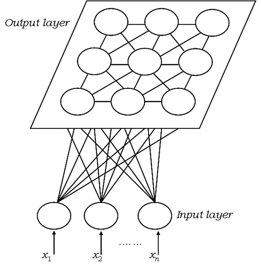
SOM representation is different from other neural networks. SOM has one input layer and one output layer: there are no hidden layers. All the neurons in the input layer are connected to all the neurons in the output layer. Input layer feeds incoming information [represented as arbitrary multidimensional vectors xi��] to output layer neurons. Each output neuron has a weights vector mi�� associated with it. These weights vectors have the same dimension as the input vectors and are often referred to as model or codebook vectors. The codebook vectors are adjusted during training so that they are as close to the input vectors as possible whilst preserving topographic properties of the input data. We will look into how this is done in more detail in the paragraph about SOM training.

Note how the output neurons are placed on a 2D plane. In fact, SOM can be used to map the input data to 1D (neurons are aligned in line) or 3D (neurons are arranged in a cube or a toroid) maps, too. In this post we will only talk about 2D maps, which are easier to understand and also most widely used in practice. The output neuron map shown above represents [after the SOM has been trained] the topographic map of input data patterns. Each area of the output neuron map is sensitive to different data patterns.

SOM feeds input data into output neurons and adjusts the codebook vectors so that the output neurons which are closer together on the output map are sensitive to similar input data patterns: neurons which are close to each other fire together. This was a bit mouthful I know, but we will see in the next parapgraph that in practice it is not as complex as it sounds. Let’s have a look at the training algorithm which will help us understand SOM better.

Training

SOM is no different from other ANNs in a way that it has to be trained first before it can be useful. SOM is trained using unsupervised learning. In particular, SOM implements a specific type of unsupervised learning called Compettive learning. In competitive learning all the output neurons compete with each other for the the right to respond when presented a new input data sample. The winner takes it all. Usually the competition is based on how close the weights of the output neuron are to the presented input data.

In case of SOM, the criterion for winning is usually Euclidean distance, however new alternative measures arose in recent research which can achieve better results for different kind of input data. The winning neuron codebook vector is updated in a way that pulls it closer to the presented data:

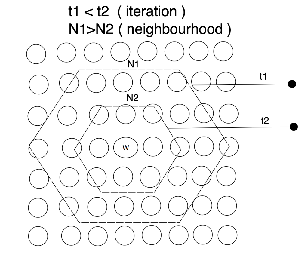
SOM takes the concept of competittve learning even further. Not only does the winning neuron gets to update its codebook vector, but so do all the neurons in its close topological neighbourhoodp. SOM neurons are thus selectively tuned: only the ones which are close to winner are updated. SOM learning is different from backpropagation where ALL [hidden and output] neurons receive the updates.

The winning neuron’s topological neighbourhood starts quite large at the beginning of the training and gradually gets smaller as the learning progresses. Naturally, you want the learning to be applied to large map regions at the start and once the neihgbouring neurons are slowly getting organized i.e. closer to the input data space, you want the neighbourhood to be shrinking.

That is all there is to the SOM learning. Obviously, the actual implementation is a bit more involved, but the above pretty much describes how SOM learns. For brevity, we can recap the SOM training in two main principles:

competitive learning: the winning neuron determines the spatial (topographic) location of other firing neurons (this places neurons sensitive to particular input dat patterns close to each other)
the learning is restricted spatially to the local neighborhood of the most active neurons: this allows to form clusters that reflect the input data space

We can now rephrase the goal of SOM training as approximation of input data into a smaller set of output data (codebooks vectors) so that the topology of input data is preserved (only the neurons close together on the output map have their codebook vectors adjusted). In other words, SOM approximates the input data space to output data space whilst repserving the data topology: if the input data samples are close to each other in the input space their approximation in the output space should be close, too.

Properties

Once the SOM is trained, its codebook vectors distribution reflects the variation (density) of the input data. This property is akin to Vector Quantization (VQ) and indeed SOM is often referred to as special type of VQ. This property makes SOM useful for lossy data compresion or even simple density estimation.

We know that SOM preserves the topology of input data. Topology retention is an excellent property. It allows to find clusters in high dimensional data. This makes SOM useful for organizing unordered data into clusters: spatial location of neuron in output corresponds to a particular domain (feature) in input. Clusters help us identify regularities and patterns in data sets.

By organizing data into clusters, SOM can detect best features inherent to input: it can provide a good feature mapping. Indeed, codebook vectos are often referred to as feature map and SOM itself is often called Self-organizing feature map.

The list of use cases does not stop there. The number of SOM output neurons is often way smaller than the number of input data samples. This basically means that SOM can be regarded as a sort of factor analysis or better, a sort of data projection method. This is indeed one of its biggest use cases. What’s even better is that SOM projection can capture non-linearities in data. This is better than the Principal Components Analysis, which as we learnt previously cannot take into account nonlinear structures in data since it describes the data in terms of a linear subspace.

Let’s finish up our incomplete list of SOM features, with something more “tangible”: data visualization. Preserving a topography of the input space and projecting it onto a 2D map allows us to inspect high dimensional data visually when plotting the output neuron map. This is extremely useful during the exploratory data analysis when are getting familiar with an unknown data set. Equally, exploring the known data set projected on SOM map can help us spot patterns easily and make amore informed decisions about the problems we are trying to solve.

Go implementation

Uh, that was a lot of theory to digest, but remember without knowing how things work, you would not be able to build them. Building, however leads to reinforcing and deeper understanding of theoretical knowledge. That’s the main reason I have decided to take on SOM as my next side project in Go: I wanted to understand it better. You can find my full implementation of SOM in Go on Github or if you want to start hacking straight away, feel free to jump into godoc API documentation.

Let’s have a look at the simplest example about how to use the gosom to build and train Self-organizing maps. The list of steps is pretty straight forward. You create a new SOM by specifying a list of configuration parameters. SOM has both data (codebook) and map (grid) properties and we need to configure the behaviour of both. Let’s start with map configuration. SOM map is in gosom implementation called Grid. This is how you create a SOM grid configuration:grid configuration

1 2 3 4 5 6 // SOM configuration grid := &som.GridConfig{ Size: []int{2, 2}, Type: "planar", UShape: "hexagon", }

We need to specify how big of a grid we want our map to have. The above example chooses a map of 2 x 2 output neurons. Of course the real life example would be bigger. The size of the grid depends on the size of the data we want the SOM to be trained on. There has been a lot of articles written about what is the best size of the grid. As always, the answer is: it depends 🙂. If you are not sure or if you are just getting started with SOM, the som package provides GridSize function that can help to make the initial decision for you. As you get more familiar with SOM, you can also inspect the output of TopoProduct function which implements Topographic Product, one of the many SOM grid quality measures.

Next we specify the Type of a grid. At the moment the package only supports a planar type i.e. the package allows to build 2D maps only. Finally, a unit shape UShape is specified. Output neurons on the map are often referred to as “units”. The package supports hexagon and rectangle unit shapes. Picking the right unit shape often has a large effect on the SOM training results. Remember how the neighbourhood of the winning neuron determines which other neurons gets training? Well in case of hexagon we have up to 6 potential neighbours, whilst in case of recatngle we only have 4. All in all, choosing hexagon almost always provides better results due to larger neihgbourhood of winning neurons.

Next we proceed to codebook configuration. There are two simple parameters to be specified: Dim and InitFunc:codebook configuration

1 2 3 4 cb := &som.CbConfig{ Dim: 4, InitFunc: som.RandInit, }

Dim specifies the dimension of the SOM codebook. Remember this dimension must be same as the dimension of the input data we are trying to project onto the codebook vectors. InitFunc specifies codebook initialization function. We can speed up SOM training by initializing codebook vectors to some values. You have two options here: random or linear initialization via either RandInit or LinInit functions. It has been proven that linear initialization often leads to faster training as the codebook values are initialized to the values from the linear space spanned by top few principal components of passed in data. However, often random initialization suffices.

Finally we add both configurations together and create a new SOM map:create new SOM

1 2 3 4 5 6 7 8 9 10 mapCfg := &som.MapConfig{ Grid: grid, Cb: cb, } // create new SOM m, err := som.NewMap(mapCfg, data) if err != nil { fmt.Fprintf(os.Stderr, "\nERROR: %s\n", err) os.Exit(1) }

Now that we have a new and shiny SOM, we need to train it. gosom provides several training configuration options each of which has an effect on the training results:SOM training configuration

1 2 3 4 5 6 7 8 9 // training configuration trainCfg := &TrainConfig{ Algorithm: "seq", Radius: 500.0, RDecay: "exp", NeighbFn: som.Gaussian, LRate: 0.5, LDecay: "exp", }

Let’s go through the parameters one after another. gosom implements two main SOM training algorithms: sequential and batch training. Sequential training is slower than the batch training as it literally, like the name suggests, goes through the input data, one sample after another. This is arguably one the main reasons why SOM haven’t been as largely adopted as I would expect. Luckily, we have an option to use batch algorithm. Batch algorithm splits the input data space into batches and trains the outpu neurons using these batches. batch algorithm approximates the codebook vectors of output neurons as weighted average of codebook vectors in some neighbourhood of the winning neuron. You can read more about the batch training here. Go’s easy concurrency makes it an excellent candidate for batch training implementation.

Chosing an appropriate training algorithms does not come without drawbacks! Whilst batch training is faster, it merely provides a reasonably good approximation of SOM codebooks. Sequential training will always be more accurate, but often the results provided by batch training are perfectly fine for the problem you are trying to solve! My advice is: experiment with different options and see if the produced results are good enough for you.

Next few configuration parameters are sort of interrelated. Radius allows you to specify initial neihbourhood radius of the winning neuron. Remember, this neighbourhood must be shrinking as we progress through the training. At the beginning we want the neighbourhood to be as large as possible, ideally so that it covers at least 50% of all output neurons and as the training progresses, the neighbourhood gradually shrinks. How fast does it shrink is defined by RDecay parameter. You have the option of chosing either lin (linear) or exp (exponential) neighbourhood decay. NeighbFn specifies a neihbourhood function that lets you calculate the winning neuron neighbourhood i.e. it calculates the distance radius of the winning neuron to help you identify the neighbours which should receive the training. Again, you have several options available to you, have a look into the documentation.

Finally, LRate parameters defines a learning rate. This controls the amount of training each neuron should receive during the different stage of the training. At the beginning we want the training to be as large as possible, but as we progress through and our data is getting more organized, we want the amount of training the neurons receive to be shrinking – there is no point to pour water into a full bucket :-). Just like Radius, LRate also lets you define how fast should the learning rate be shrinking. Again, the right options depend on your use case, but starting in the range of 0.5-0.2 is a pretty good choice

Now that we understand training parameters better, we can start training our SOM. We need to provide a data stored in a matrix and number of training iterations. Number of training iterations depends on the size of the data set and its distribution. You will have to experiment with different values.training

1 2 3 4 if err := m.Train(trainCfg, data, 300); err != nil { fmt.Fprintf(os.Stderr, "\nERROR: %s\n", err) os.Exit(1) }

Once the training finishes, we can display the resulting codebook in what’s called U-matrix. UMatrix function generates a simple umatrix image in a specified format. At the moment only SVG format is supported, but feel free to open a PR if you’d like different options :-)u-matrix

1 2 3 4 if err := m.UMatrix(file, d.Data, d.Classes, format, title); err != nil { fmt.Fprintf(os.Stderr, "\nERROR: %s\n", err) os.Exit(1) }

Finally, gosom provides an implementation of a few SOM quality measures that help you calculate quantization error, which measures the quality of the data projection. You can use QuantError function for this. Som topography can be quantified by calculating its topopgraphy error and topography product available via TopoError and TopoProduct functions.

Examples

gosom provides two simples examples available in the project’s repo. The examples both demonstrate the practical uses of the package as well as the correctness of training algorithm implementations. Let’s have a look at one of the examples which is sort of a “schoolbook” example of using SOM for clustering data. Let’s generate a “pseudo-chaotic” RGB image and try to sort it’s colors using SOM. The code to generate the image is pretty simple:create messy RGBA image

1 2 3 4 5 6 7 8 9 10 11 12 13 14 15 16 17 18 19 20 21 22 23 24 25 26 27 28 29 30 31 32 33 34 func main() { // list of a few colors colors := []color.RGBA{ color.RGBA{255, 0, 0, 255}, color.RGBA{0, 255, 0, 255}, color.RGBA{0, 0, 255, 255}, color.RGBA{255, 0, 255, 255}, color.RGBA{0, 127, 64, 255}, color.RGBA{0, 0, 127, 255}, color.RGBA{255, 255, 51, 255}, color.RGBA{255, 100, 67, 255}, } // create new 40x40 pixels image img := image.NewRGBA(image.Rect(0, 0, 40, 40)) b := img.Bounds() for y := b.Min.Y; y < b.Max.Y; y++ { for x := b.Min.X; x < b.Max.X; x++ { // choose a random color from colors c := colors[rand.Intn(len(colors))] img.Set(x, y, c) } } f, err := os.Create("out.png") if err != nil { log.Fatal(err) } defer f.Close() if err = png.Encode(f, img); err != nil { log.Fatal(err) } }

This will generate an image that looks sort of like this:

It’s a pretty nice pixel chaos. Let’s use SOM to organize this chaos into clusters of different colors and display it. I’m not going to show the actual code to do this as you can find the full example in the Github repo. SOM training data is encoded into a matrix of 1600x4 . Each row contains R.G.B and A color values. If we now use SOM to cluster the image data and display the resulting codebook on the image we will get something like this:

We can see that the SOM created nice pixel clusters of related colors. We can also display u-matrix which looks as below and which basically confirms the clusters visible in the color image shown above:

This concludes our tour of gosom. Feel free to inspect the source code and don’t hesitate to open a PR 🙂

Conclusion

Thank you for reading all the way to the end! I hope you enjoyed reading this post at least as much as I enjoyed writing it. Hopefully you have even learnt something.

We talked about Self-organizing maps, a special kind of Artificial Neural Network which is useful for non-linear data projection, feature generation, data clustering, data visualization and in many more tasks.

The post then introduced project gosom, SOM implementation in Go programming language. I explained its basic usage on a simple example and finished by showing its usage on sorting colors in a “chaotic” image.

Self-organizing maps are a pretty powerful type of ANN which can be found in use in many industries. Let me know in the comments if you come up with any interesting use case and don’t hesitate to open a PR or issue on Github.

Fun With Neural Networks in Go

My rekindled interest in Machine Learning turned my attention to Neural Networks or more precisely Artificial Neural Networks (ANN). I started tinkering with ANN by building simple prototypes in R. However, my basic knowledge of the topic only got me so far. I struggled to understand why certain parameters work better than others. I wanted to understand the inner workings of ANN learning better. So I built a long list of questions and started looking for answers.

“I have no special talents. I am only passionately curious.” – Albert Einstein

This blog post is mostly theoretial and at times quite dense on maths. However, this should not put you off. The theoretical knowledge is often undervalued and ignored these days. I am a big fan of it. If nothing else, understanding the theory helps me avoid getting frustrated with seemingly inexplicable results. There is nothing worse than not being able to reason about the results you program produces. This especially more important in machine learning which is by default an ill-posed maths problem. This post is merely a summary of the notes I made when exploring ANN learning. It’s by no means a comprehensive summary. Nevertheless, I hope you will find it useful and maybe you’ll even learn something new.

If you find any mistakes please don’t hesitate to leave a comment below. I will be more than happy to learn from you and address any inaccuracies in the text. Let’s get started!

Artificial Neural Networks (ANN)

There are various kinds of artificial neural networks. Based on a task particular ANN performs we can roughly divide them into the following groups:

Regression – ANN outputs (predicts) a number based on input data
Robotics – ANN uses sensor outputs as inputs and produces some output[s]
Vision – ANN processes digital images trying to understand them in some way
Optimization – ANN finds the best set of values to solve some optimization problem
Classification – ANN classifies data into arbitrary number of predefined groups
Clustering – ANN clusters data into groups without any apriori knowledge

In this post I will only focus on classification neural networks which are often referred to simply as classifiers. More specifically, I will talk about Feedforward ANN classifiers. Most of the concepts I will discuss in this post are applicable to other kinds of ANN, too. I will assume you have a basic understanding of what a Feedforward ANN is and what components it consists of. I will summarize the most important concepts on the following lines. If you want to dig in more depth, there is plenty of resources available online. You can see an example of a 3-layer feedforward ANN on the image below:

The above feedforward network has three layers: input, hidden and output. Each layer has several neurons: 44 in input layer, 44 in hidden layer and 22 in the output layer. Feedforward neural network is a fully connected network: all the neurons in neighbouring layers are connected to each other. Each neuron has a set of network weights assigned which serve to calculate a weighted input (let’s mark it as z) to the neuron’s activation function. You can see how this works if we zoom in on nne neuron:

From the image above it should be hopefully obvious that network weights allow to control the output of particular neuron (activation) and thus the overall behaviour of the neural network. Input neurons have unit weights (i.e. each weight is equal to 11) and their activation function is [often] what’s referred to as identity function. Identity activation function simply “mirrors” the neuron input to its output i.e. . The feedforward network shown on the first image above has two output neurons; it can be used a simple binary classifier. ANN classifiers can have arbitrary number of outputs. Before we dive more into how the ANN classifiers work, let’s talk a little bit about what a classification task actually is.

Note: The above mentioned ANN diagram doesn’t make the presence of neural network bias unit obvious. Bias unit is present in every layer of feedforward neural network. Its starting value is often set to 11, although some research documents that initializing the bias input to a random value from uniform Gaussian distribution with μ=0�=0 (mean) and σ=1�=1 (variance) can do just fine if not better. Bias plays an important role in neural networks! In fact, bias units are at the core of one of the most important machine learning algorithms. For now, let’s keep in mind that bias is present in every layer of feedforward neural network and plays an important role in neural networks.

Classification

Classification can be [very] loosely defined as a task which tries to place new observations into one of the predefined classes of objects. This implies an apriori knowledge of object classes i.e. we must know all classes of objects into which we will be classifying newly observed objects. A schoolbook example of a simple classifier is a spam filter. It marks every new incoming email either as a spam or not spam. Spam filter is a binary classifier i.e. it works with two classes of objects: spam or not spam. In general we are not limited to two classes of objects; we can easily design classifiers that can work with arbitrary number of classes.

Note: In practice, most spam filters are implemented using Bayeseian learning i.e. using some advanced Bayesian network or its variation. This does not mean that you can’t implement spam filter using ANN, but I thought I’d point this out.

In order for ANN to classify new data into a particular predefined class of objects we need to train it first. Classifiers are often trained using supervised learning algorithms. Supervised learning algorithms require a labeled data set. Label data set is a data set where each data sample has a particular class “label” assigned to it. In case of spam filter we would have a data set which would contain a large number of emails each of which would be known in advance to be either spam or not spam. Learning algorithm adjusts neuron weights in hidden and output layers so that the new input samples are classified to the correct group. Supervised learning algorithms differ from “regular” computer science algorithms in way that instead of turning inputs into outputs they consume both inputs and outputs and “produce” parameters that allow to fit new inputs into outputs:

Learning algorithm literally teaches the ANN about different kinds of objects so that it can eventually classify newly observed objects automatically without any further help. This is exactly how we as humans learn, too. Someone has to tell us first what something is before we can make any conclusion about something new we observe. If you dive a little bit into neuroscience you will find out that our brain is a very powerful classifier. Classification is a skill we are born with and we often don’t even realize it. Take for example how often do we refer to insect as flies, mosquitos etc. We hardly ever use their real biological names. It’s too costly for our brain to remember the name of every single object in the world. Our brain classifies these objects into existing groups automatically without our too much thinking. Before this happens automatically we are “trained” (taught), so that our brain doesn’t classify flies as something like airplanes.

Backpropagation

Neural network training is a process during which the network “learns” neuron weights from a labeled data set using some learning algorithm. There are two kinds of learning algorithms: supervised and unsupervised. ANN classifiers are often trained using the former, though often the combination of both is often used in practice. This blog post will discuss the most powerful supervised learning algorithms used for training feedforward neural networks: Backpropagation.

Behind every learning (not just ANN learning) is a concept of reward or penalty. Either you are rewarded when you learnt something (measured by answering particular set of questions) or you are penalized if you didn’t (failed to answer the question or answered it incorrectly). Backpropagation, like many other machine learning algorithms, uses the penalty approach. To measure how good the ANN classifier is we define a cost function sometimes referred to as objective function. The closer the output produced by ANN is to the expected value, the lower the value of the cost function for a particular input is i.e. we are penalized less if we produce correct output.

At the core of the backpropagation algorithm is partial derivative of the cost function with respect to its weights and biases i.e. Backpropagation effectively measures how much the cost changes with regards to changing network weights and biases. Neural networks are quite complex and understanding how they work can be challenging. Backpropagation summarises the overall ANN behavior in a few simple equations. In this sense backpropagation provides a very powerful tool to understand ANN behavior.

I’m not going to explain how backpropagation works in this post in too much detail. There is plenty of resources available online if you want to dig more into it. In a gist, backpropagation calculates errors in outputs of neurons in each network layer all the way back from the output layer to the output of the first hidden layer. It then adjusts the weights and biases of the network (this is the actual learning) in a way that minimizes the error in the output layer computed by the cost function . The error of the output layer is the most important one for the result, but we need to calculate the errors of each particular layer as these errors propagate through the network and thus affect the network output.

I would encourage you to dive more into the underlying theory. There is a real geeky calculus beauty to the algorithm which will give you a very good understanding of one of the most important machine learning algorithms out there. Instead of explaining the algorithm in much detail, I decided to summarize it in two points which I believe are the most crucial for understanding the behavior of feedforward neural network classifiers:

Cost function is a function of the output layer i.e. it is a function of output neuron activations.
Learning slows down if any of the “input” neurons is “low-activation”, or if any of the “output” neuron has saturated.

The first point should hopefully be pretty intuitive from the earlier network diagram. We push some input through the network, which produces some output by the output layer neurons. This output is used to calculate the error (cost) with regards to the expected output (label) acccording to the chosen cost function.

Let’s zoom in at the second point: learning slowdown. Learning slowdown, in the context of ANN, means the slowdown of the network weights (and bias) change during the run of the training algorithm. Like I said before, backpropagation changes the network weights with regards to the calculated error for given input and expected output. Change of the weights is the core of the learning. When the weights stop changing during backpropagation, the learning stops as the cost no longer changes, hence we can improve the output of the network. By doing a little bit of calculus we could show that backpropagation learning depends on derivation of the activation function. We could sum this up using a simple equation below:

where is the cost function, ain is the activation (i.e. the output produced by the neuron) of neuron that is an input to network weight of another neuron in the next layer and is the error of the neuron output from the weight. The picture below should give you a better idea about the equation above:

We could further show that the error depends on a derivation of the activaion of the intermediary neuron in the output produced by neuron with weights (remember derivation is always defined in some point – in our case that point is output produced by a particular neuron). The most important implication of this equation for network learning is that the change of cost with regards to change of weights depends on the activation input into weight and on activation function derivation in the point equal to output of the neuron with weights. Clearly, activation function plays a crucial role in how fast the neural networks can learn, so it’s a topic worth exploring further.

One of the most well known activation functions is sigmoid function often referred to simply as sgmoid. Sigmoid is well known to be used in logistic regression. Sigmoid holds some very interesting properties which make it a natural choice of neuron activation function in ANN classifiers. If we look closely on the sigmoid function on the graph below we can see that it resembles a continuous approximation of step function found in transistor switches which can be used to signal binary output (on or off). In fact, we could show that by tuning sigmoid parameters we could get a pretty good approximation of the step fuction. The ability to simulate a simple switch with boolean behavior is handy for classifiers which need to decide whether the newly observed data belongs to a particular class of objects or not.

I mentioned earlier that if the output neuron saturates then the network stops learning. Saturation means there is no rate change happening which means the derivative in any saturation point is ≈0≈0. This means that the partial derivation of cost function by weights in the equation mentioned earlier tends to get to ≈0≈0. This is exactly the case with sigmoid function. Notice on the graph above how sigmoid eventually saturates on 00 . Sigmoid suddenly doesn’t seem like the best choice for the activation function, at least not for the network output neurons. Luckily, by choosing a particular kind of cost function we can subdue the effect of neuron saturation to some degree. Let’s have a look at what would such cost function look like.

Cost function and neuron activations

Cost function is a crucial concept for many machine learning algorithms, not just backpropagation. It measures the error of computed output for a given input with regards to expected result. Cost function output must be non-negative by definition. As I will show you later on, good choice of the cost function can hugely improve the performance of ANN learning whilst a bad choice can lead to suboptimal results. There are several kinds of cost functions available. Probably the most well known one is quadratic cost function.

Quadratic cost function calculates mean squared error (MSE) for a given input and expected output:

where is the number of training samples, is the desired output, represents the number of layers in ANN, so is the activation of the output layer neuron for a particular input.

Whilst MSE is suitable for many tasks in machine learning, we could prove that it’s not the best choice of the cost function for ANN classifiers. At least not for the ones that use the sigmoid activation in the output layer. The main reason for that is that this combination of activation and cost can slow down ANN learning.

We could, however, show by performing a bit of calculus that if the output neurons are linear i.e. their activation function is defined, then the quadratic cost function will not cause learning slowdown and thus it can be an appropriate choice of cost function. So why don’t we ditch the sigmoid and go ahead with the linear activations and quadratic cost function combination instead? It turns out linear activations can still be pretty slow in comparison to other activation functions we will discuss later on.

So what should we do if our output layer neurons use sigmoid activation function? We need to find a better cost function than the quadratic cost, which will not slow down the learning! Luckily, there is one we can use instead. It’s called cross-entropy function.

Cross-entropy cost function

Cross-entropy is one of the most widely used cost functions in ANN classifiers. It is defined as follows:

It’s important to point out that if you do decide to use the cross entropy cost function you must design your neural network in the way that contains as many outputs as there are classes of objects. Additionally the expected outputs should be mapped into one-of-N matrix. Having this in mind, you can start seeing some sense in the cross entropy function. Befor I explain in more defatil that cross-entropy cost addresses the problem of learning slowdown when using the sigmoid activation, I want to highlight some important properties it holds:

it’s a non-negative function (mandatory requirement for any cost function)
it’s a convex function (this helps to prevent getting stuck in local minimum during learning)

Notice that if yk=0��=0 for some input then the first term in the above equation sum addition disappears. Equally if yk=1��=1 the same thing happens with the second term. We can therefore break down the cross-entropy cost function into following definition:

where y� is expected output and a� is neural network output. Plotting the graphs for both cases should give us even better understanding.

In the first case we are expecting the output of our network to be y=1�=1. The further the ANN output is from the expected value (11), the higher the error and the higher the cost output:

In the second case, we are expecting the output of our network to be y=0�=0. The closer the output of our network is to the expected output (00), the smaller the cost and vice versa:

Based on the graphs above we can see that cross-entropy tends to converge towards zero the more accurate the output of our network gets. This is exactly what we would expect from any cost function.

Let’s get back to the issue of learning slowdown. We know that at the heart of the backpropagation algorithm is a partial derivative of cost function by weights and biases. With a bit of calculus we can prove that when using cross-entropy as our cost function and sigmoid for activation in the output layer, the resulting partial derivative does not depend on the rate of change of activation function. It merely depends on the output produced by it. By choosing the cross-entropy we can avoid the learning slowdown caused by the saturation of the sigmoid activation function.

If your output neurons use sigmoid activation it’s almost always better to use corss-entropy cost function.

Hyperbolic tangent activation function (tanh)Before we move on to the next parargraph, let’s talk shortly about another activation function whose properties are similar to the sigmoid function: hyperbolic tangent, often referred to simply as tanh. Tanh is in fact just a rescaled version of sigmoid. We can easily see that on the plot below:

Similar to the sigmoid, tanh also saturates, but in different values: −1−1 and 11. This means you might have to “normalize” the output of the tanh neurons. Once your tanh outputs are normalized you can use the cross-entropy cost function in backpropagation algorithm. Some empirical evidence suggests that using tanh instead of sigmoid provides better results for some learning tasks. However, there is no rigorous proof that tanh outperforms sigmoid neurons, so my advice to you would be to test both and see which one performs better for your particular classification task.

Softmax activation and log-likelihood cost function

By using cross-entropy function in combination with sigmoid activation we got rid of the problem with saturation, but the learning still depends on the output of the activation function itself. The smaller the output the slower the learning gets. We can do better as we will see later on, but first I would like to talk a little bit about another activation function which has found a lot of use in ANN classifiers and in deep neural networks: softmax function, often referred to simply as softmax. Softmax has some interesting properties that make it an appealing choice of the output layer neurons in ANN classifiers. Softmax is defined as below:

ai=ezi∑nk=1ezk��=��∑�=1��

where ai�� is activation of i�-th neuron and zi�� is input into activation of i�-th neuron. The denominator in the softmax equation simply sums “numerators” across all neurons in the layer.

It might not be entirely obvious why and when should we use softmax instead of sigmoid or linear activation functions. As always, the devil lies in the details. If we look closely at the softmax definition, we can see that each activation ai�� represents its proportion with regards to all activations in the same layer. This has an interesting consequence for the other neuron activations. If one of the activations increases the other ones decrease and vice versa i.e. if one of the neurons is dominant, it “subdues” the other neuron outputs. In other words: any particular output activation depends on all the other neuron activations when using the softmax function i.e. particular neuron output no longer depends just on its weights like it was the case with sigmoid or linear activations.

Softmax activations of all neurons are positive numbers since the exponential function is always positive. Furthermore, if we sum softmax activations across all neurons in the same layer, we will see that they add up to 11:

∑i=1nai=1∑�=1��=1

Given the above described properties we can think of the output of softmax (by output we mean an array of all softmax activation in particular network layer) as a probability distribution. This is an excellent property to have in ANN classifiers. It’s very convenient to think of an output neuron activations as a probability that particular output belongs to a particular class of objects. For example we can think of ai�� in the output layer as an estimate of the probability that the output belongs to the i�-th object class. We could not make such assumption using sigmoid function as it can be proved that the sum of all activations of sigmoid function in the same layer does not always add up to 11.

We have shown earlier that by clever choice of cost function (cross-entropy) we can avoid learning slowdown in ANN classifiers when using sigmoid activations. We can pull the same trick with softmax function. Again, it will require a different cost function than the cross-entropy. We call this function log-likelihood. Log-likelihood is defined as below:

C=−log(aLyk)�=−��(��)

where L� is the last network layer and yk�� denotes that the expected output is defined by class k�.

Just like cross-entropy, log-likelihood requires us to encode our outputs into on-of-N matrix. Let’s have a closer look at this cost function like we did with cross-entropy. The fact that the output of softmax can be thought of as a probability distribution tells us two things about the cost function:

The closer the particular output is to the expected value is, the closer its output is to 11 and the closer the cost tends to get to 00.
The further the particular output is from the expected value, the closer its output is to 00 and the cost tends to grow to infinity.

The log-likelihood behaves exactly like we would expect the cost function to behave. This can be seen on the plot below:

So how does softmax address learning slowdown? By performing a bit of calculus we could once again show that partial derivative of log-likelihood by weights (∂C∂w∂�∂�), which is a at the core of backpropagation algorithm, merely depends on the output produced by activation output just like it was the case with sigmoid and cross-entropy. In fact, softmax activation and log-likelihood perform quite similar as sigmoid and cross-entropy. So when should you use which one? The answer is it depends. A lot of influential research in ANN space tends to use softmax and log-likelihood combo which has a nice property if you want to interpret the output activations as probabilities of belonging to a particular class of objects.

Rectifier linear unit (ReLU)

Before we move on from the topic of activation functions, I must mention one last option we have at our disposal: rectifier linear unit, often referred to simply as ReLU. ReLU function is defined as follows:

f(x)={x0ififx>0x≤0�(�)={��>00��≤0

ReLU has been an active subject of interest of ANN research. Over the years it has become a very popular choice of activation function in deep neural networks used for image recognition. ReLU is quite different from all the previously discussed activation functions. As you might have noticed on the plot above, ReLU does not suffer from saturation like tanh or sigmoid functions as long as its input is greater than 00. When the ReLU input is negative, the ReLU neurons stop learning completely. To address this, we can use a similar function which is a variation of ReLU: Leaky ReLU (LReLU).

LReLU is defined as follows:

f(x)={xaxififx>0x≤0�(�)={��>0��≤0

where a� is a small constant which “controls” a slope of LReLU output for the case of negative values. The actual value of the constant can differ for different use cases. The best I can advise you is to experiment with different values and pick the one that gives you the best results. LReLU provides some improvement in learning in comparison to the basic ReLU, however the improvement can be negligible. Worry not, there seems to be a better alternative.You can find plots of both ReLU and LReLU on the picture below:

A group of Microsoft researchers achieved some outstanding results in image recognition tasks using another variation of ReLU called Parametric Rectifier Linear Unit (PReLU). You can read more about the PReLU in the following paper. You will find out, PReLU is just a “smarter” version of LReLU. Whilst LReLU forces you to choose the slope constant c� before you kick off the learning, PReLU can learn the slope constant c� during backpropagation. Furthermore, whilst LReLU slope constant is static i.e. it stays the same for all neurons during the whole training, PReLU can have different slope values for different neurons at different states of the training!

The question now is, which one of the ReLU activations should we use? Unfortunately there does not seem to exist any rigorous proof or theory about how to choose the best type of rectifier linear units and for which tasks it is the most suitable choice of neuron activation. The current state of knowledge is based heavily on empirical results that show that rectifier units can improve the performance of restricted boltzman machines, acoustic models and many other tasks. You can read more about evaluation of different types of rectifier activation function used in convolutional networks in the following paper.

Weights initialization

Choosing the right neuron activations with appropriate cost function can clearly influence the performance of ANN. But we can go even further. I found out during my research the network weights initialization can play an important role in the speed of learning. This was a bit of a revelation to me. I would normally go ahead and initialize all neuron weights in all hidden layers to values from Gaussian distribution with 00 mean and standard deviation 11 without too much thinking. It turns out there is a better way to initialize the weights which can increase the speed of learning!

So what is wrong with choosing μ=0�=0 and σ=1�=1 parameters of Gaussian distribution I mentioned earlier? Imagine a situation when a significant number of neuron inputs are ≈0≈0. This is not an unusual situation. As you could see earlier, sigmoid or ReLU can easily produce values ≈0≈0 if the neurons inputs are ≪0≪0. When that’s the case, the weighted output of the neurons (i.e. the input into the neuron activation function) in the next layer can produce values of Gaussian distribution whose standard deviation is ≫0≫0 (the actual value depends on number of neurons). The problem with large standard deviation of activation input is that it causes the saturation of the neuron outputs. As we learnt earlier this has a consequence of learning slowdown.

We can avoid this problem by choosing a better set of Gaussian distribution parameters for weight initialization. There is no exact formula what should the standard deviation of weight initialzation be, but some research suggests that by choosing the standard deviation to be around the inverse of the square root of number of input weights (≈1/n−−−√≈1/�) should give you better performance than the uniformly distributed values I mentioned at the beginning of this discussion. If we plot the values of both network weights distributions for both cases it could look something like the plot below:

You should spot straight away that the distribution we are aiming for is much sharper i.e. its bell curve is much steeper. Low standard distribution helps to avoid neuron saturation and speeds up ANN learning, which is what we are striving for. You may have noticed that I did not mention how to initialize weights of bias neurons. It turns out, the weights initialization of bias neuron does not play any significant role in ANN learning so it should be ok to stick to the original standard deviation 11 without worrying too much.

Learning optimization

The goal of ANN learning algorithm is to find network weights for which the output of the cost function is as minimal as possible. This is clearly an optimization problem: we need to find weights that niminimize the output of the cost function. One of the most famous optimization algorithm used to solve this problem is called gradient descent. I’m not going to discuss the gradient descent algorithm here. Again, there is plenty of resources online if you want to understand it. And I would strongly advise you to do so, as gradient descent has huge number of applications, not only in machine learning.

Instead, I would like to mention some alternative solutions. In particular, I would like to talk shortly about some advanced optimization algorithms you can use instead of gradient descent. There are several options available at our disposal. Probably the most well known is Broyden–Fletcher–Goldfarb–Shanno, often referred to simply as BFGS and its limited memory alternative L-BFGS. Another alternative would be Conjugate gradient.

Why do I mention these advanced optimization methods? First of all, majority people are well aware of the gradient descent and so was I when I started doing my research. At some point I came across Yann LeCun’s paper on efficient backpropagation which discusses them in broader detail. These algorithms can seem very complicated, but their efficient implementations are available in many numerical toolboxes. Their biggest advantage is they don’t require much tuning. At least not as much as gradient descent. There is no need to pick many parameters except for number of iterations we want to run them for. They just work and if implemented properly they often outperform gradient descent. They are often more suitable choice for large machine learning problems which deal with huge data sets than gradient descent. If these algorithms are so good why do so many people still rely on good old gradient descent or any of its variations?

The answer, as it often is in the world of science (or life in general), is the complexity. Like I already mentioned, some of these algorithms are quite advanced and not easy to understand for some people. This can make their debugging quite hard. Often their implementations differ between various toolboxes which makes their debugging even harder. Finally, gradient descent performance is often acceptable and much better understood. It’s good to be aware that these algorithms exist and are available to use.

Neural networks in Go

Armed with the newly gained knowledge I could finally have a better understanding of neural networks. But I didn’t want to stay in theory. After all a certain wise man once said something which I find incredibly true:

“What I can not create I do not understand” – Richard Feynman

I’ve been a big fan of Go language for a while and I wondered on and off how well does it perform in numerical computations. After doing a bit of research I found the awesome gonum project that contains a great wealth of numerical packages. I took them for a spin and to my great joy, I found out that the gonum packages are pretty damn fast as long as you take advantage of the vectorised operations. Gonum is one of the biggest gems in the Go ecosystem, so do not hesitate and spend some time exploring the packages in it – you won’t regret!

The result of my hacks is a small project. I am well aware of the awesome projects like go-ml or golearn and many many others. The main reason why I decided create my own implementation despite many a people discouraging me as it being a waste of time was for purely learning experience and therefore the project itself should therefore be treated accordingly 🙂 You might find it useful and maybe it will even inspire you to hack on your own, improved implementation. The learning experience I got from this was priceless!

Conclusion

We have finally reached the end of the post. Thank you very much for reading! It’s been a long ride! We learnt about various techniques that can help us speed up ANN learning. We learnt about learning slowdown and how we can address it by choosing appropriate combination of neuron activations and cost function. Based on the research I’ve done, it seems the most popular choice of neuron activation function in classification tasks is some varioation of ReLU for the hidden layer neurons (to model system’s non-linearities) and softmax activation for the output layer neurons. The presence of softmax in the output layer “dictates” the use of log-likelihood cost function. As always, YMMV and the particular choice might differ based on the taks your network performs. All you need to do is to roll up your sleeves and make some experiments.

Writing this blog post has been amazing personal journey for me. It made me revisit some old knowledge of neural networks theory and learn tonnes of new stuff from many research papers I had not heard of before. I hope you have enjoyed reading thist post as much as I have writing it. If you have any comments, do not hesitate to leave them below.

Principal Component Analysis – Part 2

This is the second post of the series about Principal Component Analysis (PCA). Whilst the first post provided a theoretical background, this post will discuss the actual implementation of the PCA algorithm and its results when applied to some example data.

Theory Recap

In the first post we learnt that PCA looks for a vector basis that can express the analysed data in a better (less redundant) way, whilst retaining as much information from the original data as possible. The vectors that form this vector basis are called *principal components**.

We learnt that the princpal components point the direction of highest variance. The hope behind this thinking is that the variance along a small number of principal components (i.e. less than the number of measurement types) provides a reasonably simplified model of the complete data set.

Finally, we learnt that PCA assumes that the principal components are orthogonal which makes finding them a problem solvable using linear algebra.

Eigenvectors and diagonal matrix

The previous post introduced a concept of covariance matrix as an important construct that can help to reveal signal and noise in our data. The solution to finding principal components takes advantage of some of the properties covariance matrix exhibits.

We know that covariance matrix is a square symmetric matrix. We also know that in ideal case the covariance matrix should be a diagonal matrix with variances on its diagonal and all the off-the diagonal values equal to zero. The solution to PCA lies in finding a way that diagonalizes the covariance matrix.

From linear algebra we know that for a symmetric matrix S�, we can find a matrix E� such that the following equation holds true:

S=EDET�=��

where matrix D� is a diagonal matrix and E� is a matrix that contains eigenvectors of matrix S� stored in its columns. Eigenvectors always come in pairs with eigenvalues. Whilst the eigenvectors of covariance matrix carry the information about the direction of the highest variance, eigenvalues provide a measure of its proportion. Put another way: the higher the eigenvalue of the eigenvector the more information can be found in its direction.

Let’s go back to the original matrix equation PCA tries to solve:

XB=X′��=�′

where X� is the data matrix we are trying to express using the vector basis stored in the columns of matrix B�. The result of the transformation is a new matrix X′�′.

Let’s create a covariance matrix CX′��′ from matrix X′�′ i.e. the covariance matrix of the transformed data set. Let’s assume that each column of X′�′ is mean-centered so we can express CX′��′ as follows:

CX′=1nX′TX′��′=1��′��′

We can rewrite this equation using X� like this:

CX′=1n(XB)T(XB)=BT(1nXTX)B��′=1�(��)�(��)=��(1��)�

We can see that the covariance matrix of the transformed data can be expressed using the covariance matrix of the original data matrix:

CX′=BTCXB��′=��

We also know that CX�� is a symmetric matrix, so the previous formula can be be express like this:

CX′=BTCXB=BT(EDET)B��′=��=��(��)�

If we now choose the matrix B� so that it contains eigenvectors of covariance matrix CX�� in its columns, i.e. B=E�=�, we can show that CX′��′ is diagonal:

CX′=D��′=�

This result takes advantage of an important property of eigenvectors: ET=E−1��=�−1. Since we chose B� so that B=E�=� we can prove the correctness of the previous equation as follows:

CX′=BT(EDET)B=ETEDETE=(E−1E)D(E−1E)=D��′=��(��)�=��=(�−1�)�(�−1�)=�

We can see that the principal components can be found by finding the eigenvectors of the covariance matrix of the measured data. This finally concludes our quest for finding the principal components.

Algorithm

Armed with this knowledge we can finally formalize the PCA algorithm in a simple step by step summary:

Construct the data matrix; each row contains separate measurement
Mean center each column of data matrix
Calculate the covariance matrix from the data matrix
Calculate the eigenvectors and eigenvalues of the covariance matrix
Sort the eigenvectors by the largest eigenvalue
Profit 🙂

Before we go ahead and apply this algorithm on some example data sets, we will shortly discuss some alternative solutions.

Singular Value Decomposition (SVD)

Singular value decomposition is a matrix diagonalization algorithm. It allows to express a matrix in the following form:

X=UΣV�=�Σ�

where ΣΣ is a diagonal matrix with non-negative numbers on its diagonals and columns of matrices U� and V� are orthogonal. We call the vectors in U� and V� left and right singular vectors respectively. Principal components are the right singular vectors.

We are not going to be discussing SVD in more detail in this post. Just remember that you can use SVD to find the principal components, too. In fact the PCA and SVD are so closely related that the two are almost interchangeable. We will demonstrate this on a practical example later in this post.

Mean square error minimization

Another framework derives the PCA by using its property of minimizing the mean squared error. This is often framed as a projection error problem. In this case, we define a loss (error) function:

J(x)=1n∑k=1n∥xk−x′k∥2�(�)=1�∑�=1�‖��−��′‖2

where xk�� are the data measurements, and x′k��′ are defined as follows:

x′k=∑i=1q(eTixk)ei��′=∑�=1�(��)��

where vectors ei�� are the orthonormal basis we are trying to find in a way that minimizes the distance between the original data and their projections into the new vector space. Put another way: we are trying find some orthonormal basis ei�� that minimizes the loss function J(x)�(�).

THere is an interesting research happening in this field. Turns out you can do projection without actual PCA. ## Examples

It’s time to take the PCA algorithm for a spin and apply it on some data. We will start with the data set described in the first post. You can download it from my repo on GitHub here. The repo also contains the PCA implementation source code in R.

First thing we need to do is to mean center the raw data. Sometimes you will also have to perform feature scaling on the collected data. This is often required when the values of measured features vary by large degree such as when your matrix contains measurements in different units like kilometers and milimeters. By performing feature scaling you make sure that each data feature contributes to the result by approximately the same proportion. Our test data does not require the feature scaling.

You can see the comparison of raw and mean centered data at the following plot:

In the next step we will calculate the covariance matrix from the mean centered data:

CX=[1.37600.88300.88301.0474]��=[1.37600.88300.88301.0474]

We can notice that the off-the diagonal items are non-zero, which means that the two features in our data are correlated. This means that we should be able to reduce the dimension of this data set!

We now need to calculate the eigenvectors and eigenvalues of the covariance matrix. If you use the R language to calculate these, you can use a handy function called eigen(). This function automatically orders the eigenvectors based on the size of their eigenvalues. You should get the following results:

eigenvalues=[2.10987820.3135314]eigenvectors=[−0.7690815−0.63915070.6391507−0.7690815]��=[2.10987820.3135314]��=[−0.76908150.6391507−0.6391507−0.7690815]

To illustrate that the eigenvectors of the covariance matrix really do highlight the directions of highest variance we will overlay our mean centered data with regression lines defined by the both found eigenvectors:

The above rendered plot shows that the eigenvectors are orthogonal to each other like we expected. More importantly, we can see that the line which is defined by the eigenvector with the bigger eigenvalue shows a strong pattern in the data: it approximates the direction of runner’s movement. The second eigenvector “carries” less information. It basically tells us that some data points fluctuate around the line that is parameterized by the first eigenvector.

We will now try to find the principal components using SVD and compare the results to our eigenvector driven algorithm. We know that the principal components are equal to the right singular vectors. When we calculate the SVD of our covariance matrix and look at the matrix V� which contains the right singular vectors we should see the following result:

V=[−0.7690815−0.6391507−0.63915070.7690815]�=[−0.7690815−0.6391507−0.63915070.7690815]

The column vectors of V� are [almost] exactly the same as the eigenvectors of the covariance matrix we found earlier. The only difference is the sign of the second right singular vector. This does not matter as long as the calculated vectors are orthogonal to each other. Flipping the sign of the vector merely flips its direction to the exact opposite side and has no effect on the variance. This should be obvious from the plot we drew earlier.

Principal components are the vector basis that allows to express the original data in a better way than they were collected. Let’s illustrate this by plotting the data expressed using the new vector basis. We will use our well know matrix transformation equation:

XB=X′��=�′

Let’s show the comparison between the original and transformed data by drawing a simple plot:

We can see that expressing the original data using the principal components rotated it in a way that describes it better. Principal components transformed the data captured on a camera from some arbitrary angle so that it now highlights the runner’s trajectory. It should be clear that the important information lies along x� axis and the y� values captured by camera are rather redundant and can be removed without losing too much information.

Dimensionality reduction

Dimensionality reduction using PCA is a straightforward task once we know how much information are we willing to lose. This obviously depends on many factors, but in our example we can only reduce the dimension by a single degree. We can measure the information loss by calculating the proportion of lost variance. There are two ways to go about it:

measure the mean square transformation (projection) error
measure the proportion of variance captured by particular eigenvalue

In the first case we would calculate the projection error using the following formula:

Error=1m∑mi=1∥x(i)−x(i)proj∥21m∑mi=1∥x(i)∥2��=1�∑�=1�‖�(�)−��(�)‖21�∑�=1�‖�(�)‖2

where x� is our mean centerd data and xproj�� is the projected data. The upper index (i)(�) is a number of dimensions we decided to keep.

The second case can be formalized using following equation:

VARcap=∑mi=1(eig2i)∑nk=1(eig2k)��=∑�=1�(��2)∑�=1�(��2)

where VARcap�� is a proportion of variance captured by particular eigenvalues eigi��. In our example we would find out that the first principal component (the one with the highest eigenvalue) captures 97.84% of variance. We will accept the ~2% information loss and go ahead and reduce the data dimension in our example. We will use the same transformation equation, but instead of using both principal components we will only use the first one. The result will be a one dimensional matrix i.e. a single column vector.

So now that we know how to transform the data and how to measure the data loss, it’s time to learn how to reconstruct the original data back. Thi is actually pretty simple. All we need to do is to solve our familiar matrix equation:

X=X′B−1=X′BT�=�′�−1=�′��

We know that X� contains mean centered data so if we wanted to reconstruct the raw data we would need to add the original mean values of particular features to the result of this equation. We will not peform the full reconstruction from the transformed data. Instead, we will look at reconstrucing the data from the reduced data set. Once we do this, we can plot the results for comparison:

The above plot nicely illustrates the loss of one dimension. Whilst the variance along the eigenvector with the highest eigenvalue has been kept, the data along the second eigenvector has completely disappeared! As we learnt, reducing the data dimension naturally causes data loss. Luckily, according to our previous calculation, this loss is only about 2%. In reality, you would strive for much smaller data loss.

Digital image compression

Before we conclude this post we will have a quick look at one more example which involves digital image processing. We will run the PCA algorithm on some arbitrary image downloaded from the internet:

The size of the image is 400×320400�320 pixels. For simplicity, we have only used one of the three RGB dimensions. We will now try to find the principal components and perform the dimensionality reduction.

Once we found the principal components we can plot the relatinship between retained proportion of variance and number of principal components:

We can see that that the image data can be reasonably well explained by just a few principal components, maybe 6 or 7. These capture over 95% of data variance, which should be good enough for machine processing. Let’s display the compressed image, using the data captured by top 7 principal components:

We can identify the person in the picture. This is pretty good, given that we only used 400×7400�7 data measurements. which gives us 97.8% data compression of the original data! This means significant processing time gain!

Whilst this result can be good enough for machines, it is not great for the presentation purposes or for any practical tasks done by humans. We can’t properly see all the face features. If we want better precision we need to increase the number of principal components used for compression. We can experiment with different compression levels and compare the results in the graph below:

We can see that even the single top principal component does identify the main patterns in image, however the projection is very poor. Using 7 vectors, as we mentioned earlier, gets pretty close, but not great. The higher the number of principal components we use the higher the data variance and better the resulting picture.

Conclusion

In this post we formalized the PCA algorithm in a step by step guide. We have then looked at some practical examples that. First we removed the redundant dimension from the runner’s data and illustrated the importance of eigenvectors. Then we looked at how can we reconstruct the original data from the transformed data set. Finally, we showed how PCA can be used for simple image compression.

I would like to thank you for spending your free time reading this post. gIt was a good fun and learning experience writing it. I hope you enjoyed it and if you spotted any inaccuracies, feel free to leave a comment below.

You can find all the source code in my GitHub repo

Principal Component Analysis – Part 1

This is the first of the two post series about Principal Component Analysis (PCA). This post lays down important knowledge bricks that are needed to understand the core principles of the PCA algorithm. The second post will discuss the actual implementation and its results by applying it to various data sets.

Motivation

The world is becoming more data driven than ever before. We collect large amounts of data from arbitrary sources. This is often because we don’t know which data best describes the systems we are trying to understand. The fear of missing out on capturing important features forces us to collect a lot of redundant data.

Amassing large amounts of data introduces a whole new set of problems. For starters, the more data we collect, the longer it takes to process it. We also find it hard to understand big data sets as we naturally try to visualize them. Visualizing is impossible when the collected data goes beyond three dimensions. Luckily, there has been a lot of research done over the years focused on a lot of big data issues. Principal Component Analysis is one of many algorithms which can help us when making sense of big piles of data.

Introduction

Principal Component Analysis (PCA) is one the most well known pattern recognition algorithms. It provides a nonparametric way to identify hidden patterns in complicated data sets. Applying PCA to a complex data set can reveal simple structures that often underlie it. PCA also allows to express the data in a simpler way that can highlight its most important features.

PCA is often used during Exploratory data analysis, but the most well known use of PCA is dimensionality reduction. The algorithm can uncover correlated features hidden inside confusing data sets. These features can be often removed or replaced with their simpler representations without losing too much information. This results in smaller amounts of data which leads to shorter processing times. Removing redundant data features also provides for another interesting PCA application: data compression.

It is important to stress that PCA will not yield useful results for all data sets! In this series of posts we will show you some practical applications of PCA, but we will also discuss some of the use cases where PCA is not the most suitable algorithm to apply when looking for interesting patterns in data.

Intuition

Imagine we are recording a runner on a running track using an old camera from some arbitrary angle. The runner runs from one point to another and back until she gets tired and stops. For illustration purposes we will be using an ancient camera, which has a tiny sampling rate of 5Hz. To make things even simpler, we will also assume the runner is not fit and is only capable of 10s of intensive run. This will give us 50 pictures (10s ×× 5Hz). Each picture provides a pair of x� and y� coordinates on 2D plane. Altogether during our experiminet we will capture 100 data points.

Unless the runner had a few drinks beforehands, her trajectory should be a straight line. As we mentioned earlier, our camera captures a pair of coordinates for each picture it takes. The captured data however do not provide the most efficient way to describe the run. The reason why we make this statement will hopefuly become more obvious by looking at graphs drawn from the recorded data. Let’s create a simple scatter plot to get a better idea abou the runner’s trajectory:

There are two things we can spot straight away from the plot. First, the camera angle is not perpendicular to the running track, so the collected data points are a bit rotated around the x� axis. We can also notice, by drawing a simple regression line over the plotted data points, that there is a clear correlation between x� and y� coordinates captured by our camera:

We should be able to figure out the parameters of the regression line from the captured data. This would allow us to calculate y� from x� and vice versa with some reasonable precision. Now we can hopefullysee that our data set contains redundant information which does not provide any benefit. A single data point per measurement should be enough to describe the run. We will now try to use the PCA algorithm to identify and remove these data redundancies.

You can find the source code to the above plots in my GitHub repo

Problem definition

Now that we are hopefully a bit more familiar with the practical issues PCA tries to solve, we will try to formalize them as a mathematical problem. Once we find a solution to this problem, we will codify it in our favourite programming language. Many Machine Learning algorithms require some knowledge of Linear algebra, Calculus and Statitiscs. PCA is no different. This article assumes the reader has at least basic understanding of the above listed topics.

We will start by expressing the measured data as a matrix X�. Each row of the matrix X� will hold a separate pair of measured coordinates. The matrix will have 50 rows (one row per measurement) and 2 columns (one column for each coordinate). You can see the first few rows of matrix X� below:

X=⎡⎣⎢⎢⎢⎢3.3815634.5278752.655682⋮3.3891135.8541784.411995⋮⎤⎦⎥⎥⎥⎥�=[3.3815633.3891134.5278755.8541782.6556824.411995⋮⋮]

We know from linear algebra that each pair of coordinates our camera captured represents a two dimensional vector which lies in some vector space of the same dimension. We also know that any vector space is defined by its vector basis, sometimes called vector space generators. Vector space basis is a maximal set of linearly independent vectors that can generate the whole vector space via their linear combination. Put another way: every vector in particular vector space can be expressed as a linear combination of the vector space basis.

Let’s consider some basic two dimensional basis vectors b1�1 and b2�2. Let’s further assume b1�1 and b2�2 are a othornormal basis. We will now lay them into some matrix B� by columns:

B=[b1b2]=[1001]�=[�1�2]=[1001]

We can express the first measurement in matrix X� using this basis like this:

x1=[3.3815633.389113]=3.381563∗b1+3.389113∗b2�1=[3.3815633.389113]=3.381563∗�1+3.389113∗�2

Every measurement in matrix X� can be expressed using the same vector basis in a similar way. We can formalize this using a simple matrix equation:

XB=X��=�

It’s worth noting that expressing the data via the orthonormal basis does not transform it. This is an important property of orthogonal data projection – idempotency:

XB=X=(XB)B��=�=(��)�

We now know that our measurements lie in the vector space defined by the vector basis [b1,b2][�1,�2]. The problem with the basic basis is that it is often not the best basis to express your data with. If we look at the plot we have drawn earlier we can see that the basic basis, which point in direction of the plot coordinate axis, is not in line with the camera angle from which we were recording the runner’s movement. If it were, the plotted data points would fluctuate around x� axis pointing in the direction of the runner’s trajectory. The basic vector basis reflects the method we gathered the data, not the data itself!

Is there a different vector basis which is a linear combination of the basic basis that best expresses our data?

Answering this question is the goal of PCA. If such basis exists, expressing our data using this basis will transform (rotate) the original data in a way that describes it in a way that can highlight its important features. We can formalize this goal using the following matrix equation:

XB′=X′��′=�′

where matrix X′�′ contains the transformed data, matrix B′�′ holds the new vector basis in its columns just like matrix B� held the basic vector basis. If we look closely at this equation, we will notice that there is nothing surprising about it. It merely formalizes the data transformation using the new vector basis.

XB′=⎡⎣⎢⎢x1x2⋮⎤⎦⎥⎥[b′1b′2…]��′=[�1�2⋮][�1′�2′…]

X′=⎡⎣⎢⎢x1∗b′1×2∗b′1⋮x1∗b′2×2∗b′2⋮……⎤⎦⎥⎥�′=[�1∗�1′�1∗�2′…�2∗�1′�2∗�2′…⋮⋮]

Each row of matrix X′�′ contains a particular data row of matrix X� expressed in the new basis. It’s also worth pointing out that the idempotency property mentioned earlier still holds true on the transformed data:

X′B′=X′=(X′B′)B′�′�′=�′=(�′�′)�′

We have now formalised our goal to a search for a new vector basis that can re-express our original data different way. This new set of vector basis are the principal components we are looking for.

We still do not know based on what criterias do we choose the new basis. The answer to this question turns out to be quite simple: information. Put another way: the new vector basis should transform the original data in a way that retains as much information about the original data as possible.

Information retention

Our task is to find a data transformation that will retain as much information of the original data as possible. We can measure the information present in arbitrary data sets by a well known signal to noise ratio(SNR) defined as follows:

SNR=σ2signalσ2noise��=��2��2

where $\sigma^2{signal}and��\sigma^2{noise}$ represent the variances of signal and noise in the data set.

Variance is an important statistical measure which helps us understand spread of the data in a data set. It is defined as follows:

var(X)=∑ni=1(Xi−X¯¯¯¯)(Xi−X¯¯¯¯)(n−1)=∑ni=1(Xi−X¯¯¯¯)2(n−1)��(�)=∑�=1�(��−�¯)(��−�¯)(�−1)=∑�=1�(��−�¯)2(�−1)

where X� is a vector of measurements, \overline{X} is its mean value and n� is a number of data samples in vector X�.

Variance provides a much better way to measure the information in arbitrary data sets than mean value. If we relied solely on the mean value, we would not be able to tell the difference between the following two data samples of the same length:

data1=[data2=[10010110210310410510610710181064]]��1=[��2=[10101010101010101010012345671864]]

At the first sight they seem clearly different. First data set contains only 1010s, whilst the second data set exhibits more variability. If we calculate the mean values of both samples we will get the same result: 10. This can mistakenly lead us to make the wrong assumption that the both data sets are the same. Variance, on the other hand, reveals more information about internal structure of the data we are trying to understand.

From the SNR�� formula we can see that the higher the SNR�� the more signal there is available in the data. This means that in order to retain as much information from our original data, the new vector basis we are searching for, should point in the direction of the highest variance: the higher the variance the more information we retain. If we apply this intuition to the runner’s data, we should discover that the direction of the highest variance follows the trajectory of the runner’s movement.

Covariance matrix

Variance is a pretty good statistical measure, however it is only useful for single dimensional data i.e. vectors. It does not help when we are trying to find out if there is any relationship between any types of data features in arbitrary data sets. We need a better measure that will be able to capture these relationships. Covariance provides such measure. Covariance is always measured between two arbitrary data sets of the same length. It is defined as follows:

cov(X,Y)=∑ni=1(Xi−X¯¯¯¯)(Yi−Y¯¯¯¯)(n−1)��(�,�)=∑�=1�(��−�¯)(��−�¯)(�−1)

where X� and Y� are two arbitrary vectors holding n� number of measurements and X¯¯¯¯�¯ and Y¯¯¯¯�¯ are their particular mean values. You might have noticed that if we calculate covariance with the data itself, we will get the variance:

cov(X,X)=∑ni=1(Xi−X¯¯¯¯)(Xi−X¯¯¯¯)(n−1)=var(X)��(�,�)=∑�=1�(��−�¯)(��−�¯)(�−1)=��(�)

So what does covariance actually tell us about two data sets? Its exact value is not actually as important as it is its sign:

if the sign is positive, then both data sets increase together
if the sign is negative, then both data sets decrease together
if the covariance is zero, the two data sets are independent

According to tese properties two data sets are correlated ONLY IF their covariance is non-zero. If we now calculate the covariance between the two columns in the runner’s data matrix we will notice that the resulting value is positive. This confirms our suspicion about the relationship between the collected coordinates: our data set really is redundant.

Covariance is helpful when dealing with two dimensional data. But what if we are trying to figure out a possible relationship in data sets that span larger number of dimensions? We use covariance matrix which is defined as follows:

CX=1nXTX��=1��

where n� is a number of rows (measurements) of matrix X�. Note that the data columns of matrix X� have been “mean centered” as per the covariance formula! The importance of mean centering is discussed in several scientific papers – for the purpose of this article all of our data are mean centered [according to the definition of covariance].

Covariance matrix is extremely valuable as it carries the information about relationships between all measurements types stored in particular column vectors of our data matrix. This might not be obvious from the formula, so let’s have a look at a simple example to understand this better. Let’s consider a three dimesional data matrix (i.e. the matrix has 3 columns) to illustrate some important properties of the covariance matrix. The example data matrix Y� will hold three different types of measurements in its column vectors x�, y� and z�. Let’s also assume that data stored in each of these vectors have already been mean centered:

Y=[xyz]�=[��]

If we now calculate its covariance matrix CY�� we will get the following result:

CY=1n(xyz)T(xyz)=1n⎛⎝⎜xyz⎞⎠⎟(xyz)=⎛⎝⎜cov(x,x)cov(y,x)cov(z,x)cov(x,y)cov(y,y)cov(z,y)cov(x,z)cov(y,z)cov(z,z)⎞⎠⎟��=1�(��)�(��)=1�(��)(��)=(��(�,�)��(�,�)��(�,�)��(�,�)��(�,�)��(�,�)��(�,�)��(�,�)��(�,�))

The properties of the covariance matrix should now be more obvious:

covariance matrix is a square symmetric matrix of size n×n�×� where n� is a number of data measurements
diagonal terms are the variances of particular measurement types which carry the signal
off-the diagnoal terms are the covariances between particular measurement types which signify the noise

We know that the bigger the variance, the higher the signal. We also know that non-zero covariance signifies the presence of the noise (in form of data redundancies). In light of this knowledge we can now rephrase our goal to finding a new vector basis which maximises variance and minimises covariance of the trasnformed data set features.

In the most idealistic scenario, we would like the PCA to find the new vector basis so that the covariance matrix of the transformed data is diagonal i.e. its off-the diagonal values are zero. There is one subtle assumption PCA makes about the new basis: the new vector basis is orthogonal. Orthogonality makes finding the new basis fairly easy task solvable with linear algebra. We will discuss this more in the next part of this series where we formalize the PCA algorithm in simpe steps.

Conclusion

In this blog post we have laid down the most important knowledge bricks for understanding Principal Component Analysis. We learnt that the PCA tries to find a new vector basis that transforms the original data to a new data set in a way that maximizes variances of particular measurement types and at the same time minimizes covariances between them.

The new vector basis points in a direction of the highest variances. Orthogonality of the new vector basis assumption puts a restriction on the basis direction: imagine playing an old arcade game like pacman where you can only move your character in direction of right angles.

In the next part of this series we will look into the actual implementation of PCA. We will then apply it to our simple two dimensional example of runner’s data. Finally we will look at more complex multidimensional data like digital images and show a simple data compression algorithms based on PCA.

Acknowledgements: Thanks to Kushal Pisavadia for reading the first draft of this post and providing valuable feedback.

tf.cond: simple lambdas

tf.cond: parametrised lambdas

tf.while_loop: basics

tf.while_loop: fixed number of iterations

tf.while_loop: conditional break

Summary

TensorFlow Dataset API Exploration Part 1

Dataset API quick rundown

Creating Datasets

from_tensor_slices()

from_tensors()

Summary

Hopfield Networks in Go

Human memory

Hopfield network

Energy and pattern basins

Open questions

Capacity and spurious patterns

Memory recall

Go implementation

Recovering MNIST images

Conclusion

Self-organizing Maps in Go

Motivation

Introduction

Representation

Training

Properties

Go implementation

Examples

Conclusion

Fun With Neural Networks in Go

Artificial Neural Networks (ANN)

Classification

Backpropagation

Cost function and neuron activations

Cross-entropy cost function

Softmax activation and log-likelihood cost function

Rectifier linear unit (ReLU)

Weights initialization

Learning optimization

Neural networks in Go

Conclusion

Principal Component Analysis – Part 2

Theory Recap

Eigenvectors and diagonal matrix

Algorithm

Singular Value Decomposition (SVD)

Mean square error minimization

Dimensionality reduction

Digital image compression

Conclusion

Principal Component Analysis – Part 1

Motivation

Introduction

Intuition

Problem definition

Information retention

Covariance matrix

Conclusion

Supporters